Attention is a foundational concept in deep learning, especially in transformers like BERT and GPT. Google’s team published the scholarly document “Attention is all you need“, which made ChatGPT possible.
Attention is a mechanism that allows models, particularly neural networks, to focus on specific parts of an input sequence while processing it. In simple terms, attention scores different parts of an input based on their relevance to a given task, allowing the model to prioritize important information over irrelevant details. This is particularly useful in handling long sequences, where treating all inputs equally would be computationally expensive and inefficient.
Why is this important? If it is in embeddings, imagine you need to find another embedding that would be your next paragraph, for example. Transformer, with attention, makes that decision.
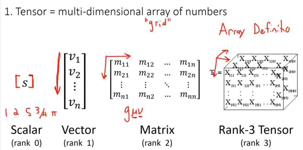
Tensor graphically
I suggest reading this article, as it nicely explains scalars, vectors, tensors – and matrices. A tensor is often viewed as a generalized matrix.

Source: Rodolphe Vaillant’s homepage.
Tensors in Attention
Since deep learning models work with numerical data, attention mechanisms use tensors (multi-dimensional arrays) to perform computations. Value (V) is the main focus, and we need the next Value (V), output, the prediction of what is next. Below are the key tensors involved in attention:
When you input a sentence, it gets tokenized and mapped to an embedding tensor:
- Each paragraph/text/word (token) is converted into a fixed-size vector.
- These vectors are stacked into a 2D tensor of shape (sequence_length, embedding_dim).
- If you use batching, the tensor shape is (batch_size, sequence_length, embedding_dim).
For example, for the batch of 2 sentences, each with five words, and an embedding size of ada-002 ChatGPT 1536 dimensional vector:
X = Tensor ( 2, 5, 1536)
Each number in this tensor represents some learned numerical feature of a token.
Batch Size
Batch size refers to the number of samples processed together in a single forward and backward pass during training or inference in machine learning and deep learning models. It is a critical hyperparameter that impacts the model’s performance, memory usage, and convergence speed.
Type 1: Small Batch Size (e.g., 1–32 samples)
- Requires less memory.
- Provides more frequent updates to model weights, leading to faster convergence.
- Introduces more noise due to high variance in gradient updates, which can improve generalization but may also slow training.
Type 2: Large Batch Size (e.g., 128–4096 samples)
- Takes advantage of hardware parallelism (e.g., GPUs, TPUs).
- More stable and accurate gradient estimates, reducing noise.
- May require a lower learning rate to prevent overshooting.
- Can lead to poor generalization if too large (e.g., overfitting to training data).
Type 3: Mini-Batch Gradient Descent (Typical Choice)
- A middle ground between stochastic gradient descent (SGD, batch size = 1) and full-batch gradient descent (batch size = entire dataset).
- Provides a balance between computational efficiency and training stability.
Small batch sizes allow for better generalization but take longer to train. Large batch sizes speed up training but may lead to poor generalization or require fine-tuned learning rate schedules.
Query, Key, and Value (Q, K, V) Tensors
- Query (Q): The representation of the current input (or token) that is trying to find relevant information.
- Key (K): The representation of all inputs (or tokens) in the sequence that could provide relevant information.
- Value (V): The actual data that is retrieved when a key is matched with a query.
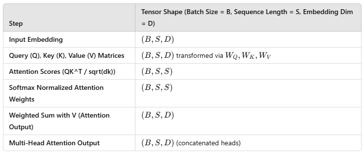
The above tensors are matrix shapes (batch size, sequence length, embedding dimension).
These are computed using learnable weight matrices:
Q = X WQ , K = X WK, V = X WV
Where:
- WQ, WK, WV are learnable weight matrices of shape (embedding_dim, hidden_dim).
- Q, K, V tensors now have the shape (batch_size, sequence_length, hidden_dim).
Attention Scores (QKT)
The attention mechanism computes similarities between the Query and Key tensors by taking their dot product:
Attention Scores = Q ⋅ KT / √dk
This results in a matrix of shape:
(sequence length, sequence length)
where each entry represents how much attention one token should pay to another. T = transpose it has the same dimension for tensors to calculate, in other words, shape from (batch_size, sequence_length, hidden_dim) to (batch_size, hidden_dim, sequence_length), making it compatible for matrix multiplication via (hidden_dim, hidden_dim). The division dk helps stabilize the gradient.
The output shape is (batch_size, sequence_length, sequence_length), representing how much each token attends to every other token.
Softmax Normalization
To convert these raw attention scores into probabilities, we apply a softmax function:
Attention Weights = softmax(Q⋅KT)
This ensures that the sum of attention weights for each query token is 1 (means across each row), making it interpretable as a probability distribution.
Weighted Sum with Values
Finally, the attention weights are multiplied with the Value (V) tensor to obtain the final attended representation:
Output = Attention Weights ⋅ V
This produces the final representation of each token, incorporating information from other relevant tokens.
The shape remains (batch_size, sequence_length, hidden_dim).
Multi-Head Attention (MHA)
Instead of using a single attention mechanism, modern architectures use multiple “heads” to compute attention in parallel. This allows the model to capture different relationships between words.
- Each head has its own Q, K, V tensors, learned separately, meaning each head has its own Q, K, V matrices.
- The outputs of all heads are concatenated and transformed to form the final output, in other words, the outputs are concatenated and projected using another weight matrix.
- Final shape: (batch_size, sequence_length, embedding_dim).
Why Are Tensors Crucial in Attention?
Efficient Computation – Matrix multiplications allow attention to be computed efficiently in parallel using GPUs.
Scalability – Tensors generalize attention across different batch sizes and sequence lengths.
Differentiability – Since all operations are tensor-based, the entire attention mechanism is differentiable, making it trainable using backpropagation.
Summary of Tensors in Self-Attention:

Key Takeaways
✔ Transformers operate on tensors, applying matrix operations for self-attention.
✔ Each token is converted into tensors (Q, K, V), processed via dot-product attention.
✔ Multi-head attention uses multiple parallel transformations.
✔ Everything is differentiable, making it trainable via backpropagation.
Let’s take the example code in PyTorch :
You can use Google Collab to run this code; it will work as you see it.
import torch
import torch.nn.functional as F

# Dummy input (batch_size=1, seq_length=5, embedding_dim=8)
X = torch.rand(1, 5, 8)

# Weight matrices
W_q = torch.rand(8, 8)  # (embedding_dim, hidden_dim)
W_k = torch.rand(8, 8)
W_v = torch.rand(8, 8)

# Compute Q, K, V
Q = X @ W_q  # (1, 5, 8)
K = X @ W_k
V = X @ W_v

# Compute attention scores
scores = Q @ K.transpose(-2, -1) / (8 ** 0.5)  # (1, 5, 5)

# Softmax normalization
attention_weights = F.softmax(scores, dim=-1)  # (1, 5, 5)

# Apply attention weights to V
attention_output = attention_weights @ V  # (1, 5, 8)

print(attention_output.shape)  # Should be (1, 5, 8)
print("Weight Tensor W")
print(W_q)
print("Attention Weights")
print(attention_weights)
print("Attention Output")
print(attention_output)
print("Tensor Query")
print(Q)
The output:
torch.Size([1, 5, 8])

Weight Tensor W
tensor([[0.8441, 0.1891, 0.6117, 0.5362, 0.6732, 0.5931, 0.0609, 0.2553],
        [0.4852, 0.0127, 0.0767, 0.3195, 0.7896, 0.9788, 0.8557, 0.7840],
        [0.8977, 0.4564, 0.4997, 0.9916, 0.5998, 0.4384, 0.3557, 0.0775],
        [0.3299, 0.3087, 0.0502, 0.7260, 0.9567, 0.6299, 0.5881, 0.8600],
        [0.6027, 0.7925, 0.6060, 0.3167, 0.8004, 0.6523, 0.4284, 0.8242],
        [0.0979, 0.4495, 0.6347, 0.5302, 0.0448, 0.7771, 0.8423, 0.9253],
        [0.5484, 0.1366, 0.1234, 0.6062, 0.2074, 0.3671, 0.1548, 0.5205],
        [0.6977, 0.4186, 0.0263, 0.4705, 0.3353, 0.1851, 0.2048, 0.0087]])

Attention Weights
tensor([[[0.0548, 0.4571, 0.1555, 0.3022, 0.0305],
         [0.0277, 0.5224, 0.1236, 0.3149, 0.0113],
         [0.0235, 0.5574, 0.1044, 0.3059, 0.0088],
         [0.0231, 0.5586, 0.1059, 0.3042, 0.0082],
         [0.0441, 0.4733, 0.1425, 0.3172, 0.0228]]])

Attention Output
tensor([[[2.0523, 2.6216, 2.4315, 1.7903, 1.8593, 2.4975, 2.5933, 2.0546],
         [2.1001, 2.6634, 2.4652, 1.8018, 1.8895, 2.5317, 2.6509, 2.0693],
         [2.1190, 2.6823, 2.4744, 1.8037, 1.8987, 2.5343, 2.6613, 2.0780],
         [2.1198, 2.6828, 2.4742, 1.8054, 1.9001, 2.5343, 2.6612, 2.0784],
         [2.0669, 2.6344, 2.4454, 1.7907, 1.8674, 2.5139, 2.6190, 2.0578]]])

Tensor Query
tensor([[[2.2132, 1.0347, 1.0996, 2.1299, 1.6344, 1.6842, 0.9784, 1.4525],
         [2.3528, 1.3777, 1.0121, 2.5207, 2.2909, 2.5994, 2.2205, 2.5341],
         [2.6278, 1.7435, 1.9519, 2.4618, 2.4398, 2.6380, 1.8158, 2.3684],
         [2.7017, 1.4744, 1.3310, 2.6113, 2.9289, 2.8076, 2.2018, 2.3492],
         [1.7606, 1.0468, 1.3165, 1.6054, 1.6300, 2.1854, 1.5939, 1.9731]]])
